A Tumor-Immune Dynamical Model with Compound Therapy and Distributed Delay

定理1  系统(1)的所有解T(t), I(t), C(t), M₁(t), M₂(t)是非负且有界的.

证  对系统(1)显然有：

由非负初始条件(2)知：T(t), C(t), M₁(t), M₂(t)均是非负的. 接着根据C(t)的非负性，可以得出

从而知

故系统(1)的所有解是非负的.

下面证明系统的有界性. 首先，由系统(1)的第一个和第三个方程知：

运用比较原理可知：

类似地，由系统(1)的第四个和第五个方程知：

至此证明了T(t), C(t), M₁(t), M₂(t)是有界的. 接着，证明I(t)的有界性. 由系统(1)的第二个方程以及T(t), C(t), M₁(t), M₂(t)的有界性知存在正常数K₁和K₂使得：

从而知I(t)也是有界的. 定理证毕.

本节讨论免疫激发分布时滞为零时系统(1)的动力学性态. 此时系统(1)变为如下常微分方程：

定理2  (i)系统(3)总存在无肿瘤平衡点E₀=(0, I₀, C₀, M₁₀, M₂₀).

(ii) 如果 $I_{0}>\frac{1}{m}\left(a_{1}-\frac{q_{1} u_{1}}{\gamma_{1}}\right)$, 则系统(3)的无肿瘤平衡点E₀是局部渐近稳定的.

证  (i)首先由系统(3)的后3个方程可得：

将C₀, M₁₀, M₂₀分别代入到系统(3)的第二个方程，可得：

其中，

由A₁ > 0, A₃ < 0知方程(4)存在正根

故系统(3)总存在无肿瘤平衡点E₀=(0, I₀, C₀, M₁₀, M₂₀).

(ii) 为了研究无肿瘤平衡点E₀的局部稳定性，计算系统(3)在平衡点E₀处的雅可比矩阵为：

从而对应特征方程的根分别为：

显然，特征值λ₁, λ₂, λ₃, λ₅是负的；当λ₄ < 0时，即 $I_{0}>\frac{1}{m}\left(a_{1}-\frac{q_{1} u_{1}}{\gamma_{1}}\right)$成立，则无肿瘤平衡点E₀是局部渐近稳定的. 定理证毕.

定理3  (i) 如果 $I^{*}<\frac{1}{m}\left(a_{1}-\frac{q_{1} u_{1}}{\gamma_{1}}\right)$, 则系统(3)存在正平衡点E^*=(T^*, I^*, C^*, M₁^*, M₂^*).

(ii) 系统(3)的正平衡点E^*是局部渐近稳定的.

证  (i) 如果系统(3)存在正平衡点E^*=(T^*, I^*, C^*, M₁^*, M₂^*), 则有：

且I^*应满足下列方程：

其中：

由B₁ > 0, B₃ < 0知方程(5)存在正根

故当T^* > 0时，即 $I^{*}<\frac{1}{m}\left(a_{1}-\frac{q_{1} u_{1}}{\gamma_{1}}\right)$, 系统(3)存在正平衡点E^*=(T^*, I^*, C^*, M₁^*, M₂^*).

(ii) 下面研究正平衡点E^*的局部稳定性，计算系统(3)在平衡点E^*处的雅可比矩阵为：

从而系统(3)在E^*处的特征方程为：

其中

显然特征方程(6)有3个负的特征根：

另外两个特征根λ₄和λ₅由下述方程决定：

可得

从而知λ₄和λ₅均为具有负实部的特征根. 故正平衡点E^*是局部渐近稳定的. 定理证毕.

由定理2和定理3, 我们定义：

则可以进一步得到如下结论.

定理4  (i) 假设 $u_{1}>\frac{a_{1} \gamma_{1}}{q_{1}}$, 则系统(3)存在唯一无肿瘤平衡点E₀且局部渐近稳定.

(ii) 假设 $u_{1}<\frac{a_{1} \gamma_{1}}{q_{1}}$. 如果u₂ > Q(u₁), 则系统(3)的无肿瘤平衡点E₀局部渐近稳定；如果u₂ < Q(u₁), 无肿瘤平衡点E₀不稳定，而正平衡点E^*存在且局部渐近稳定.

证  (i) 注意到 $a_{1}-\frac{q_{1} u_{1}}{\gamma_{1}}<0$等价于 $u_{1}>\frac{a_{1} \gamma_{1}}{q_{1}}$, 由定理2和定理3可知(i)成立.

(ii) 如果 $a_{1}-\frac{q_{1} u_{1}}{\gamma_{1}}>0$, 通过计算可以得到：

故由定理2和定理3可知(ii)成立.

注1  由定理4可知，只要化疗药物浓度足够大，即 $u_{1}>\frac{a_{1} \gamma_{1}}{q_{1}}$, 肿瘤可以直接被清除；注意到化疗的副作用，可以知道u₁的增加会降低免疫细胞的浓度. 如果结合化疗和免疫治疗，使得u₂ > Q(u₁), 则可能在 $u_{1}<\frac{a_{1} \gamma_{1}}{q_{1}}$条件下，即保持较高免疫水平的条件下控制并清除肿瘤.

本节讨论系统(1)在免疫激发分布时滞不为零的情况下正平衡点处的稳定性. 参考文献[9], 本文取核函数为弱核，即K(s)=θe^-θs, θ > 0, 则相应的平均时滞为：

下面研究Hopf分支的情况. 首先引入新的变量：

系统(1)变为如下等价的常微分方程：

注意到时滞不改变平衡点的存在性，所以系统(3)的正平衡点等价于系统(7)的正平衡点 $\widetilde{E}=(\widetilde{T}, \tilde{I}, \tilde{Y}, \widetilde{C}, \widetilde{M}_{1}, \widetilde{M}_{2})$, 其中 $\widetilde{T}=\widetilde{Y}$. 此时将系统(7)在正平衡点 $\widetilde{E}$处线性化可得：

从而可得系统(8)在正平衡点 $\widetilde{E}$处特征方程对应的根

均为负根；其余3个特征根由下列方程决定：

其中：

注意到L_i(θ) > 0(i=1, 2, 3), 由Hurwitz判据可知，方程(9)的3个根都具有负实部，即正平衡点 $\widetilde{E}$局部渐近稳定的充要条件是

代入L_i(θ) > 0(i=1, 2, 3)计算可得

其中：

显然H₁ > 0, H₃ > 0.

令Δ=H₂²-4H₁H₃, 由此可知：当Δ≤0时，Q(θ)≥0在θ > 0上恒成立，则正平衡点 $\widetilde{E}$对所有时滞都局部渐近稳定. 当Δ > 0时，定义：

若H₂ > 0, Q(θ) > 0在θ > 0上恒成立，此时正平衡点 $\widetilde{E}$对所有时滞都局部渐近稳定；若H₂ < 0, 当0 < θ < θ_cr1或θ > θ_cr2时 $\widetilde{E}$局部渐近稳定，当θ_cr1 < θ < θ_cr2时正平衡点 $\widetilde{E}$不稳定.

当θ=θ_cri(i=1, 2)时，有Q(θ_cri)=0, 易知方程(9)存在一对纯虚根. 接下来根据文献[12], 只需验证Hopf分支发生的横截条件. 由(10)式可以得到：

故系统(1)在θ=θ_cri(i=1, 2)处发生Hopf分支. 依据上述讨论，给出如下定理.

定理5  (i) 如果Δ≤0, 则正平衡点 $\widetilde{E}$对所有时滞都局部渐近稳定.

(ii) 如果Δ > 0且H₂ > 0, 则正平衡点 $\widetilde{E}$对所有时滞都局部渐近稳定.

(iii) 如果Δ > 0且H₂ < 0, 则当0 < θ < θ_cr1或θ > θ_cr2时，正平衡点 $\widetilde{E}$局部渐近稳定；当θ_cr1 < θ < θ_cr2时，正平衡点 $\widetilde{E}$不稳定且在θ=θ_cri(i=1, 2)处发生Hopf分支.

注2  由定理5可以看到当平均时滞处于中间水平时系统会产生周期解，该结果与文献[9]中的结论完全不同. 在文献[9]中只存在一个Hopf分支点，并且当平均时滞较小时存在周期解. 我们认为该差异产生的原因主要在于假设免疫细胞由肿瘤激发生成的同时还依据logistic自然增长，说明免疫细胞的自然增长对该系统动力学性态有重要影响.

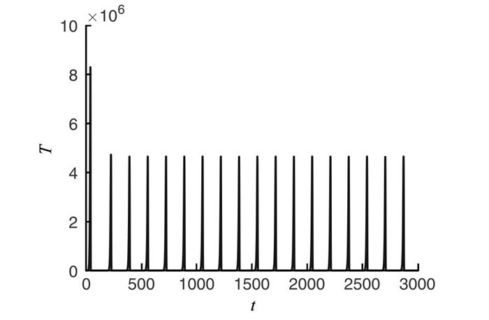
为了验证上述理论研究结果，参考文献[11]取定一组参数如下：a₁=0.43, b₁=1.02×10^-9, m=6.41×10^-12, a₂=5×10^-2, b₂=1.2×10^-11, n=2×10^-7, k=6.25×10^-6, q₁=0.8, q₂=q₃=0.6, α₁=2.08×10^-2, α₂=7.50×10⁸, β=1.2×10^-3, γ₁=0.9, γ₂=1, u₁=0.115, u₂=0.113, 计算可得系统(7)存在如下正平衡点： $\widetilde{E}=\left(2.68 \times 10^{5}, 5.12 \times 10^{10}, 2.68 \times 10^{5}, 9.63 \times 10^{9}, 0.13, 0.11\right)$. 通过计算可得临界值θ_cr1=8.66×10^-6, θ_cr2=0.47. 分别取θ₁=8.3×10^-6, θ₂=0.6, 由定理5可知，正平衡点 $\widetilde{E}$此时皆局部渐近稳定(图 1); 取θ=0.2时θ_cr1 < θ < θ_cr2, 则由定理5可知，正平衡点 $\widetilde{E}$失去稳定性，系统产生Hopf分支出现周期解(图 2).