Dynamic Analysis on a Predator-Prey Model with Mixed Migration Strategy in Advection Environments

为了使用抛物型方程的比较原理，我们将系统(2)中食饵的边界条件变为常用的Robin边界条件. 取变换u(x，t)=${\rm{e}}^{\frac{q}{d_1}x}\tilde u(x, t)$，v(x，t)= $\tilde v$(x，t)，将系统(2)转换成如下等价系统

易知系统(2)和系统(3)的解结构相同. 不失一般性，我们假设l=1.

首先考虑单物种系统

其中d，q，r＞0且b≥0. 当b∈ (0，$\frac{1}{2}$]时，令$\hat q = \sqrt {\frac{dr}{b(1-b)}} $；当b∈ ($\frac{1}{2}$，+∞)时，令$\hat q = \sqrt {4dr} $. 对于系统(4)的全局动态，根据文献[6]的定理2.1(b)和文献[10]，有如下结论成立.

引理1    设d，q，r＞0且b≥0. 关于系统(4)有如下结论：

(i) 若b＞0，则存在q^*=q^*(d，r，b)∈(0，$\hat q$)，当q∈(0，q^*)时，系统(4)存在唯一的正稳态解，记作θ(d，q，r，b)，并且是全局稳定的；当q∈[q^*，+∞)时，u=0是全局稳定的；

(ii) 若b=0，则系统(4)存在唯一的正稳态解θ(d，q，r)，并且是全局稳定的.

引理2    设d，q，r＞0且b≥0. 若系统(4)的正稳态解θ(d，q，r，b)存在，则θ(d，q，r，b)≤r.

证    首先θ(d，q，r，b)满足如下方程

当b≥1时，由强极大值原理可知θ(d，q，r，b)＜r. 现证当0≤b＜1时，θ(d，q，r，b)≤r. 令$\hat θ = \frac{θ_x}{θ} $，则

当0＜b＜1时，由强极大值原理，易知(1-b) $\frac{q}{d}$＜$\hat θ$＜$\frac{q}{d}$，并且当b=0时，有$\hat θ$ = $\frac{q}{d}$. 因为$\hat θ$ ≥(1-b)$\frac{q}{d}$，则θ_x＞0，故θ(d，q，r，b)在[0, 1]上单调递增，并在x=1处取得最大值M. 用反证法证明θ(d，q，r，b)≤r，假设M＞r，将(5)式的第一个式子在[0, 1]上积分，得

显然，总存在x₁∈[0, 1]，使得θ(x₁)=r，并且当x∈[x₁，1]时，总有θ(d，q，r，b)≥r. 将(5)式的第一个式子在[x₁，1]上积分，得

因为$\int_{x1}^{1}$θ(r-θ)dx＜0，故-bqθ(1)-dθ_x(x₁)+qθ(x₁)＞0，移项变换有

这与(1-b) $\frac{q}{d}$ ≤$\hat θ$ 矛盾，假设不成立. 因此当0≤b＜1时，θ(d，q，r，b)≤r. 证毕.

定理1    设d₁，d₂，r₁，r₂＞0且b≥0. 系统(2)存在唯一的正解(u，v)，并且正解最终有界.

证    首先，根据文献[11]，系统(3)的解局部存在且唯一，则系统(2)的解也局部存在且唯一. 其次，由最大值原理，易知u＞0，v＞0. 故只需证明解的有界性. 结合解的正性和系统(3)的第一个方程可得

根据抛物型方程的比较原理可知$\tilde u$(x，t)≤U(x，t)，其中U(x，t)满足如下方程

通过变换U(x，t)=${\rm{e}}^{\frac{q}{d_1}x}$U (x，t)，得

由引理1，2易知$\lim\limits_{t→+∞}$ U(x，t)≤r₁，故

因此，存在正常数ρ，使得0＜$\tilde u$(x，t)≤ρ. 再根据系统(3)的第二个方程，有

类似地，令V (x，t)满足

不难得到$\lim\limits_{t→+∞}$V(x，t)=r₂+c${\rm{e}}^{\frac{q}{d_1}x}$ρ，由比较原理有

因为系统(2)和等价系统(3)的解结构相同，所以系统(2)的解(u，v)最终有界. 证毕.

易见系统(2)可能存在3个边界平衡态解(0，0)，(θ(d₁，q，r₁，b)，0)和(0，r₂). 为了研究这些平衡解的稳定性，我们首先证明如下结论.

定理2    设d₁，d₂，r₁，r₂＞0且b≥0. 若(u，v)是系统(2)的解，则$\liminf \limits_{t \rightarrow+\infty}$v(x，t)≥r₂.

证   由系统(2)的第二个方程有

由比较原理易得$\liminf\limits_{t→+∞}$v(x，t)≥r₂. 证毕.

定理2表明平衡点(0，0)和(θ(d₁，q，r₁，b)，0)一定是不稳定的，下面来讨论(0，r₂)的稳定性. 考察特征值问题

其中：d，q＞0，b≥0且r∈ ${\mathbb{R}}$. 根据Krein-Rutman定理^[15]知问题(8)存在主特征值λ₁(d，q，r，b)，且对应的有严格正的特征函数ϕ₁(d，q，r，b). 结合系统(4)中的设定，根据文献[6]的引理2.1，2.2和文献[12]的命题3.1，有下列结论成立.

引理3    设d，q＞0，b≥0且r∈ ${\mathbb{R}}$. 特征值问题(8)有如下性质：

(i) 若d，r，b＞0，则存在q^*=q^*(d，r，b)∈(0，$\hat q$)，当q∈(0，q^*)时，λ₁(d，q，r，b)＞0，当q=q^*时，λ₁(d，q，r，b)=0，当q∈(q^*，+∞)时，λ₁(d，q，r，b)＜0；

(ii) 若r≤0，则λ₁(d，q，r，b)≤0，并且b=0时，λ₁(d，q，r，0)=r.

定理3    设d₁，d₂，r₁，r₂，q＞0且b≥0. 平衡解(0，r₂)的局部稳定性情况如下：

(H₁) 当r₁＞ar₂时，若b＞0，则存在q^*(d₁，r₁-ar₂，b)，使得q∈(0，q^*(d₁，r₁-ar₂，b))，(0，r₂)是不稳定的，q∈(q^*(d₁，r₁-ar₂，b)，+∞)，(0，r₂)是局部渐进稳定的；

(H₂) 当r₁＞ar₂时，若b=0，则(0，r₂)是不稳定的；

(H₃) 当r₁＜ar₂时，(0，r₂)是局部渐进稳定的.

证    系统(2)在(0，r₂)处线性化后的特征值问题如下

定义Λ为特征值问题(9)的谱，显然Λ=Λ{φ=0}∪Λ{φ≠0}. 当φ=0时，考察特征值问题

可取特征函数ψ₁(x)=1，故主特征值λ₁=-r₂＜0. 因此，对属于特征值问题(10)的特征值λ，都有Re λ＜λ₁＜0，则sup{Re λ，λ∈Λ{φ=0}}＜0. 当φ≠0时，考察特征值问题

定义σ$\left[d_\text{1} \frac{d^\text{2}} {dx^\text{2}} -q \frac{d} {dx} +r_\text{1}-ar_\text{2}\right]$为算子$d_{1} \frac{d^{2}}{d x^{2}}-q \frac{d}{d x}+r_{1}-a r_{2}$的谱，则

根据引理3，当r₁＞ar₂时，若b＞0，则存在q^*(d₁，r₁-ar₂，b)，使得q∈(0，q^*(d₁，r₁-ar₂，b))，λ₁(d₁，q，r₁-ar₂，b)＞0，则

所以(0，r₂)是不稳定的，q∈(q^*(d₁，r₁-ar₂，b)，+∞)，λ₁(d₁，q，r₁-ar₂，b)＜0，则

所以(0，r₂)是局部渐进稳定的，(H₁)成立. 类似地，当r₁＞ar₂时，若b=0，由引理3，可知λ₁(d₁，q，r₁-ar₂，b)=r₁-ar₂＞0，(0，r₂)是不稳定的，(H₂)成立. 当r₁＜ar₂时，由引理3，可知λ₁(d₁，q，r₁-ar₂，b)＜0，同样可得(0，r₂)是局部渐进稳定的，(H₃)成立. 证毕.

由定理3可知(0，r₂)的局部稳定性，下面证明若(0，r₂)是局部稳定的，则(0，r₂)是全局吸引的，从而(0，r₂)也是全局稳定的.

定理4    设d₁，d₂，r₁，r₂，q＞0且b≥0. 若条件

(C₁) r₁＜ar₂.

(C₂) r₁＞ar₂，b＞0，q∈(q^*(d₁，r₁-ar₂，b)，+∞).

之一成立，则平衡解(0，r₂)是全局稳定的.

证    由定理2有

故对∀ε＞0，存在T＞0，使得当t≥T时，有$\tilde v$(x，t)≥r₂-ε. 结合系统(3)的第一个方程，有

现考虑如下方程

由比较原理，可知当t≥T时，$\tilde u$(x，t)≤U (x，t). 通过变换U(x，t)=$\mathrm{e}^{\frac{q}{d_1} x}$U(x，t)，得

当(C₁)成立时，取ε足够小，使得r₁+aε-ar₂＜0，再由引理3得λ₁(d₁，q，r₁+aε-ar₂，b)＜0. 根据文献[10]，系统(12)的解U=0是全局稳定的当且仅当λ₁(d₁，q，r₁+aε-ar₂，b)＜0，则

当(C₂)成立时，有r₁+aε-ar₂＞r₁-ar₂＞0，由引理1可知存在q^*(d₁，r₁+aε-ar₂，b)，使得当q∈[q^*(d₁，r₁+aε-ar₂，b)，+∞)时，系统(12)的解U=0是全局稳定. 又因为(C₂)成立时，有q∈(q^*(d₁，r₁-ar₂，b)，+∞)，并且ε是任意小的正常数，所以必有q∈[q^*(d₁，r₁+aε-ar₂，b)，+∞)，故

综上所述，若(C₁)和(C₂)其中一个成立，则对∀ε₁＞0，总存在T₁＞0，使得当t≥T₁时，有$\tilde u$(x，t)≤ε₁. 结合系统(3)的第二个方程，当t≥T₁时，有

由比较原理易得

再结合(11)式和(13)式，有

可知(0，r₂)是全局吸引的，又因(0，r₂)的局部稳定性已知，所以结论成立.

在这一节中，我们使用一致持续性理论来研究系统(2)的一致持续性条件，相关理论的详细介绍可以参考文献[13].

定理5    设d₁，d₂，r₁，r₂，b＞0且r₁＞ar₂. 若q∈(0，q^*(d₁，r₁-ar₂，b))，则系统(2)是一致持续的，即存在一个正常数η，使得

证    定义P={($\tilde u, \tilde v$)∈C[0, 1]×C[0, 1]：$\tilde u$ ≥0，$\tilde v$ ≥0}，P₀={($\tilde u, \tilde v$)∈P：$\tilde u$(x)$\not \equiv$0，$\tilde v$(x)$\not \equiv$0}，∂P₀=P-P₀；定义Θ(t)为系统(3)在空间P中解的半流. 由强极大值原理可知当($\tilde u$₀，$\tilde v$₀)∈P₀时，系统(3)的解($\tilde u$(x，t)，$\tilde v$(x，t))满足$\tilde u$(x，t)＞0，$\tilde v$(x，t)＞0，故P₀是P中的开集并且还是正向不变集. 显然，∂P₀包含(0，0)，($\mathrm{e}^{\frac{q}{d 1} x}$θ(d₁，q，r₁，b)，0)和(0，r₂)；定义M_∂={($\tilde u$₀，$\tilde v$₀)∈∂P₀：Θ(t)($\tilde u$₀，$\tilde v$₀)∈∂P₀，∀t≥0}，γ(($\tilde u$₀，$\tilde v$₀))是正向轨{Θ(t)($\tilde u$₀，$\tilde v$₀)：t≥0}的极限集. 具体证明过程分为如下4步：

1) 证明$\bigcup\limits_{\left(\tilde{u}_{0}, \tilde{v}_{0}\right)\in M _\partial} \gamma\left(\left(\tilde{u}_{0}, \widetilde{v}_{0}\right)\right)$={(0，0)，($\mathrm{e}^{\frac{q}{d 1} x}$θ(d₁，q，r₁，b)，0)，(0，r₂)}.

如上所述，对∀($\tilde u$₀，$\tilde v$₀)∈M_∂，有Θ(t)($\tilde u$₀，$\tilde v$₀)∈∂P₀，即对∀t≥0，有$\tilde u$(x，t，($\tilde u$₀，$\tilde v$₀))≡0或$\tilde v$(x，t，($\tilde u$₀，$\tilde v$₀))≡0. 当$\tilde u$(x，t，($\tilde u$₀，$\tilde v$₀))≡0时，考虑如下方程

易知$\lim\limits _{t \rightarrow+\infty} \widetilde{v}(x, t)$=r₂. 当$\tilde v$≡0时，考虑如下方程

由引理1得$\lim\limits _{t \rightarrow+\infty} \tilde{u}(x, t)=\mathrm{e}^{-\frac{q}{d 1} x}$θ(d₁，q，r₁，b)或$\lim\limits _{t \rightarrow+\infty} \tilde{u}(x, t)$=0. 证毕.

2) 证明(0，0)是一个一致弱的排斥子，即对∀($\tilde u$₀，$\tilde v$₀)∈P₀，存在常数σ₁＞0，使得

使用反证法，假设(14)式不成立，则对∀σ＞0，存在一个($\tilde u$₀，$\tilde v$₀)∈P₀，使得$\limsup\limits_{t \rightarrow+\infty} $ ‖Θ(t)(($\tilde u$₀，$\tilde v$₀))-(0，0)‖＜σ，故存在t₁＞0，使得对∀t≥t₁，有‖ $\tilde u$(x，t，($\tilde u$₀，$\tilde v$₀))‖＜σ，‖ $\tilde v$(x，t，($\tilde u$₀，$\tilde v$₀))‖＜σ. 结合系统(3)的第二个方程，有

因为($\tilde u$₀，$\tilde v$₀)∈P₀，由最大值原理，可知$\tilde v$(x，t₁)＞0. 令v (x，t)是下列方程的解

这里的α＜$\tilde v$(x，t₁). 根据比较原理，当t≥t₁时，$\tilde v$(x，t)≥v(x，t). 很明显v (x，t)=$\alpha {\rm{e}}^{(r1-\sigma)(t-t1)}$是方程(15)的解. 使σ足够小以至于r₁-σ＞0，则$\lim\limits_{t→+∞}\tilde v$(x，t，($\tilde u$₀，$\tilde v$₀))=+∞，这与假设矛盾. 因此，假设不成立，{(0，0)}是P中孤立的不变集. 另外，通过类似的推导，可以证得{(${\rm{e}}^{-\frac{q}{d_1}x}$θ(d₁，q，r₁，b)，0)}是P中孤立的不变集，这里不再赘述.

3) 证明(0，r₂)是一致弱的排斥子，即对∀($\tilde u$₀，$\tilde v$₀)∈P₀，存在常数σ₂＞0，使得

使用反证法，假设(16)式不成立，则对∀σ＞0，存在一个($\tilde u$₀，$\tilde v$₀)∈P₀，使得$\limsup\limits _{t \rightarrow+\infty}$‖Θ(t)(($\tilde u$₀，$\tilde v$₀))-(0，r₂)‖＜σ，故存在t₂＞0，使得对∀t≥t₂，有‖ $\tilde u$(x，t，($\tilde u$₀，$\tilde v$₀))‖＜σ，‖ $\tilde v$(x，t，($\tilde u$₀，$\tilde v$₀))-r₂‖＜σ. 易知对∀t≥t₂，系统(2)的解(u(x，t)，v(x，t))满足‖u(x，t，(u₀，v₀))‖＜${\rm{e}}^{\frac{q}{d_1}}$σ，‖v(x，t，(u₀，v₀))-r₂‖＜σ. 结合系统(2)的第一个方程，有

使用合适的变量替换，再由比较原理可得对∀t≥t₂，有u(x，t)≥u (x，t). 其中，u (x，t)满足如下方程

定义μ₁^σ=λ₁(d₁，q，r₁-ar₂-aσ-${\rm{e}}^{\frac{q}{d_1}}$σ，b)，并且对应的特征函数为ω₁(x)＞0. 令u满足如下方程

易知u (x，t)=α₁e^{μ₁σ(t-t₂)}ω₁(x)是方程(18)的解. 其中，α₁＞0并且满足u(x，t₂)≥α₁ω₁(x)，故对∀t≥t₂，有

因为q∈(0，q^*(d₁，r₁-ar₂，b))，λ₁(d₁，q，r₁-ar₂，b)＞0. 让σ足够小，使得μ₁^σ=λ₁(d₁，q，r₁-ar₂-aσ-${\rm{e}}^{\frac{q}{d_1}}$σ，b)＞0，则$\lim\limits_{t→+∞}$u(x，t)=+∞，这与假设矛盾. 因此，假设不成立，{(0，r₂)}是P中孤立的不变集.

4) 定义连续函数D：P→ [0，+∞)，对∀($\tilde u$，$\tilde v$)∈P

由比较原理可知D^-1(0，+∞)⊆P₀. 当D(($\tilde u$，$\tilde v$))＞0或者($\tilde u$，$\tilde v$)∈P₀且D(($\tilde u$，$\tilde v$))=0时，有D(Θ(t)($\tilde u$，$\tilde v$))＞0. 根据文献[13]，称D是半流Θ(t)：P→P的一个距离函数.

由定理1，可知Θ(t)：P→P是点耗散的，又由于扩散算子的光滑性，易知半流Θ(t)：P→P是紧的. 根据文献[14]的定理2.6，Θ(t)存在一个全局的吸引子，吸引P中任意一个有界集. 因为(0，0)，(${\rm{e}}^{-\frac{q}{d_1}x}$θ(d₁，q，r₁，b)，0)和(0，r₂)是一致弱的排斥子，并且它们在P中是孤立的，即

W^S((${\rm{e}}^{-\frac{q}{d_1}x}$θ(d₁，q，r₁，b)，0))，W^S((0，0))和W^S((0，r₂))是对应于(${\rm{e}}^{-\frac{q}{d_1}x}$θ(d₁，q，r₁，b)，0)，(0，0)和(0，r₂)的稳定集. 因此，{(0，0)∪(${\rm{e}}^{-\frac{q}{d_1}x}$θ(d₁，q，r₁，b)，0)∪(0，r₂)}的子集不能在∂P₀中形成环. 根据文献[13]的定理3，总存在正常数η，使得对∀($\tilde u$₀，$\tilde v$₀)∈P₀，有

因此对∀($\tilde u$₀，$\tilde v$₀)∈P₀，存在一个正常数η使得$\liminf\limits _{t \rightarrow+\infty}$u(x，t)≥η，$\liminf \limits_{t \rightarrow+\infty}$v(x，t)≥η，结论成立. 证毕.

类似地，可以使用一致持续性理论得到系统(2)在b=0时的一致持续性，证明省略.

定理6    设d₁，d₂，r₁，r₂，q＞0且r₁＞ar₂. 若b=0，则系统(2)是一致持续的，即存在正常数η，使得

本节首先通过数值模拟验证我们的理论研究结果. 取定参数

(I) d₁=0.15，d₂=0.1，r₁=4，r₂=3，a=0.5，c=0.2，l=10.

此时r₁＞ar₂，当b=0时，由图 1(a)可知，系统对任意的q＞0都是一致持续的，该结果与定理6相符；当b=1时，由图 1(b)可知，存在一个临界的流速，使得当流速小于此临界值时，系统是一致持续的，当流速大于此临界值时，捕食者种群平均密度是3，食饵种群将会灭绝，该结果与定理4和定理5相符.

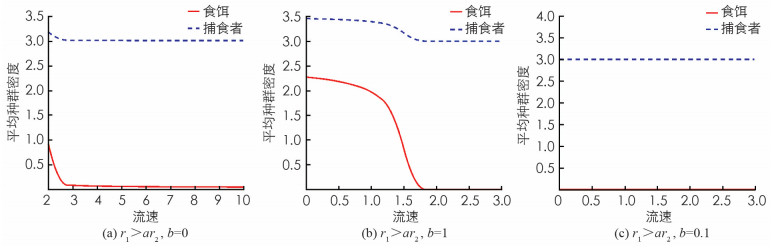
(II) d₁=0.15，d₂=0.1，r₁=1，r₂=3，a=0.5，c=0.2，l=10.

此时r₁＞ar₂，由图 1(c)可知，对任意的q＞0和b=0.1，捕食者种群平均密度总是3，食饵种群总会灭绝，该结果与定理4相符.

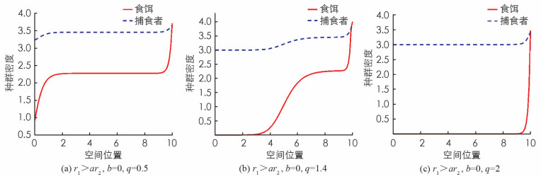
其次，我们通过数值模拟研究了不同流速对种群空间分布的影响. 选择参数组(I)，当b=0时，种群是一致持续的. 但由图 2可知，随着流速变大，种群的空间分布会发生变化，且随着流速增加食饵种群会聚集在河流的下游，由于可用资源减少，使得种群总的数量降低，因此对流的增加不利于种群的繁衍.