Stability Analysis of the Interaction Model Between Plants and Sulfides in Salt Marsh Ecosystems

考虑如下植物-硫化物的反馈模型：

其中：P=P(T)表示T时刻土壤中植物的密度，S=S(T)表示T时刻土壤中硫化物的浓度，$r P\left(1-\frac{P}{K}\right)$表示植物呈Logistic型增长，cPS表示有害的硫化物会导致植物的死亡，I_in指无植被土壤中硫化物浓度的沉积率，dS表示单位时间内硫化物浓度的衰减，bP表示植物促进硫化物浓度的增长. 模型(1)中所有的参数都是正数，其中：r表示植物的最大增长率，K是环境容纳量，c表示因硫化物引起的植物的最大死亡率，d为解毒系数即土壤中硫化物减少的系数，b表示植物促进硫化物增长的最大转化率.

为便于对模型(1)进行理论分析，我们引进以下无量纲化的变量和参数：

则模型(1)可以无量纲化为

这里：$\alpha=\frac{I_{\text {in }} c}{r^2}$, $\beta=\frac{d}{r}$, $\gamma=\frac{b c K}{r^2}$.

令$\frac{\mathrm{d} p}{\mathrm{~d} t}=\frac{\mathrm{d} s}{\mathrm{~d} t}=0$，我们发现模型(2)总是存在边界平衡点E₀=$\left(0, \frac{\alpha}{\beta}\right)$，正平衡点E^*=(p^*，s^*)=$\left(\frac{\beta-\alpha}{\beta+\gamma}, \frac{\alpha+\gamma}{\beta+\gamma}\right)$存在当且仅当β>α.

为了分析平衡点E₀和E^*的稳定性，我们在平衡点处对模型(2)进行线性化得到对应的Jocabi矩阵为

于是在E₀处，

在E^*处，

因此

于是，我们有以下定理：

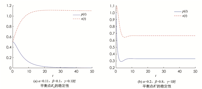
定理1  (ⅰ) 当β < α时，模型(2)只存在一个边界平衡点E₀，且E₀是局部渐近稳定的；

(ⅱ) 当β>α时，模型(2)存在两个平衡点E₀与E^*，其中E^*是局部渐近稳定的，E₀是鞍点.

引理1^[14]  (Lasalle不变原理)设在平衡点的邻域U内存在正定函数V(x)，且V(x)沿着模型(2)轨线的全导数$\dot{V}(\mathit{\boldsymbol{x}})$是半负定的. 若集合

内除平衡点外，不再包含系统的其他轨线，则模型(2)的平衡点是渐近稳定的.于是为了讨论正平衡点E^*的全局稳定性，可取Liapunov函数

因为当p>p^*时，$\int_{p^*}^p \frac{\xi-p^*}{\xi} \mathrm{d} \xi>0$，当p < p^*时，$\int_{p^*}^p \frac{\xi-p^*}{\xi} \mathrm{d} \xi=\int_p^{p^*} \frac{p^*-\xi}{\xi} \mathrm{d} \xi>0$；同理当s>s^*时，$\int_{s^*}^s \frac{\eta-s^*}{\gamma} \mathrm{d} \eta>0$，当s < s^*时，$\int_{s^*}^s \frac{\eta-s^*}{\gamma} \mathrm{d} \eta=\int_s^{s^*} \frac{s^*-\eta}{\gamma} \mathrm{d} \eta>0$. 于是V₁(p，s)>0，其中(p，s)∈U(p^*，s^*).

因为

将1-p^*-s^*=0，α+γp^*-βs^*=0代入(3)式得

于是对任意(p，s)≠(p^*，s^*)都有$\frac{\mathrm{d} V_1}{\mathrm{~d} t}<0$恒成立，因此由引理1可知模型(2)的共存平衡点E^*是全局渐近稳定的.

接下来考虑到植物和硫化物的空间扩散，我们将常微分方程模型(2)延伸至如下的反应扩散模型：

其中：p=p(x，t)，s=s(x，t)分别代表t时刻x处的土壤中植物的密度和硫化物的浓度，dΔp和Δs分别代表植物和硫化物的扩散速率，其中Δ是拉普拉斯算子，${\mathit{\Omega}} \subset \mathbb{R} $是边界光滑的有界域，模型(4)的第三个方程表示Neumann边界条件，υ是边界∂Ω上的单位外法向量，模型(4)的第四和第五个方程表示植物和硫化物的初始分布，p₀(x)和s₀(x)都是Ω上的连续函数.

设0=μ₀ < μ₁ < μ₂ < …是Ω上考虑Neumann边界条件时算子Δ的特征值.

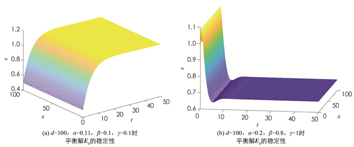
设X=$\left\{(p, s) \in\left[C^1({\mathit{\Omega}})\right]^2 \mid \frac{\partial p}{\partial \boldsymbol{v}}=\frac{\partial s}{\partial \boldsymbol{v}}=0\right\}$，将X分解为直和形式$X=\bigoplus\limits_{i=1}^{\infty} X_i$，这里X_i是特征值μ_i对应的特征空间(i=0，1，2，…).

定理2  (ⅰ) 当β < α时，模型(4)的常数稳态解E₀是局部渐近稳定的；

(ⅱ) 当β>α时，模型(4)的常数稳态解E₀是不稳定的.

证  在E₀处对模型(4)进行线性化，有

其中

这里f(ε₁，ε₂)=o(ε₁²+ε₂²)，g(ε₁，ε₂)=o(ε₁²+ε₂²).

X_i是不变子空间，并且μ_i是L在X_i上的特征值当且仅当λ_i是矩阵M_i的特征值，

于是

从而

(ⅰ) 当β < α时，tr(M_i) < 0，det(M_i)>0，λ_i^±都有负实部(i=0，1，2，…)；

(ⅱ) 当β>α时，存在μ_i使得det(M_i)＜0即λ_i^-有负实部，λ_i⁺有正实部(i=0，1，2，…)：

则

定理3  当β>α时，模型(4)的常数稳态解E^*是局部渐近稳定的.

证  对模型(4)在E^*处线性化，有

其中

这里f(ε₁，ε₂)=o(ε₁²+ε₂²)，g(ε₁，ε₂)=o(ε₁²+ε₂²).

X_i是不变子空间，并且μ_i是L在X_i上的特征值当且仅当λ_i是矩阵M_i的特征值，

于是

从而当β>α时，tr(M_i) < 0，det(M_i)>0，λ_i^±都有负实部(i=0，1，2，…)：

(ⅰ) 若[tr(M_i)]²-4det(M_i)≤0，则

(ⅱ) 若[tr(M_i)]²-4det(M_i)>0，则

因此L的特征值都具有负实部.

为了讨论模型(4)正解的全局稳定性，需要给出以下引理.

引理2  $\lim\limits_{t \rightarrow+\infty} \sup \max\limits_{\bar{{{\Omega}}}} p(x, t) \leqslant 1, \lim\limits_{t \rightarrow+\infty} \sup \max\limits_{\bar{{{\Omega}}}} s(x, t) \leqslant \frac{\alpha+\gamma}{\beta}$.

证  考虑模型

设(p(x，t)，s(x，t))是模型(4)的正解，p₁(x，t)是模型(5)的解，于是由比较原理可得

接下来考虑常微分系统

易知系统(6)的解z(t)满足$\lim\limits_{t \rightarrow+\infty} z(t)=1$，再次由比较原理可得$\lim\limits_{t \rightarrow+\infty} \sup \max\limits_{\bar{{{\Omega}}}} p(x, t) \leqslant 1$. 同理可得

定理4  当β>α时，模型(4)的常数稳态解E^*存在并且是全局渐近稳定的；当β<α时，模型(4)的常数稳态解E₀是全局渐近稳定的.

证  构造Liapunov函数

由分步积分公式以及Neumann边界条件，得

因此$\lim\limits_{t \rightarrow+\infty}$|p(x，t)-p^*|=$\lim\limits_{t \rightarrow+\infty}$|s(x，t)-s^*|=0，常数稳态解E^*关于模型(4)是全局渐近稳定的. 常数稳态解E₀的全局稳定性同上可证，只需取V₁(p，s)=V(s)=$\int_{\frac{\alpha}{\beta}}^s \frac{\eta-\frac{\alpha}{\beta}}{\gamma} \mathrm{d} \eta$即可.

取参数α>β与α < β时模型(2)与模型(4)平衡点稳定性的情况如图 1，2所示.

由图 1可知当α>β时，模型(2)的平衡点E₀是全局渐近稳定的；当α < β时，模型(2)的平衡点E^*是全局渐近稳定的. 由图 2可知取d=100，当α>β时，模型(4)的常数平衡解E₀是全局渐近稳定的；当α < β时，模型(4)的常数稳态解E^*是全局渐近稳定的.

本文在文献[1]的模型基础上稍有改动，考虑的是植被呈Logistic增长，硫化物浓度升高受土壤中硫化物的沉积以及植物的促进两方面的影响. 研究结果表明该模型的正平衡点在有无扩散的情况下都是全局稳定的，而植被的生长受多种因素的影响，因此研究营养物质与植被生长的关系也是十分有意义的.