A Parallel Finite Element Algorithm for Stokes Equations with Nonlinear Slip Boundary Conditions

空间$H^{k}(\mathit{\Omega})^{2} $的范数表示为$\|\cdot\|_{k}, L^{2}(\mathit{\Omega})^{2} $的内积与范数表示为(·，·)和‖·‖.本文所使用的空间为：

空间V的内积与范数表示为$(\nabla \cdot , \nabla \cdot ) $和$\|\cdot\|_{V}=\|\nabla \cdot\| $，定义：$ a(\boldsymbol{u}, \boldsymbol{v})=v(\nabla \boldsymbol{u}, \nabla \boldsymbol{v}), d(\boldsymbol{v}, q)=$ $(\nabla \cdot \boldsymbol{v}, q), \forall \boldsymbol{u}, \boldsymbol{v} \in V, q \in M $.本文定义字母c为一个大于0的常数，它与网格参数无关，在不同式子可代表不同值.

方程(1)的变分形式^[12]为：求$(\boldsymbol{u}, p) \in V \times M $，使得

其中$ j(\zeta)=\int_{S} g|\zeta| \boldsymbol{d} s, \zeta \in H^{\frac{1}{2}}(S)$.方程(2)等价于以下变分等式^[13]：求$(\boldsymbol{u}, p) \in V \times M $，存在且仅存在一个λ∈Λ，使得

其中凸集Λ满足：$\mathit{\Lambda}=\left\{\mu \in L^{2}(S), |\mu(x)| \leqslant 1, a, e, \text { on } S\right\} $.

假设对Ω的粗网格剖分T^H和细网格剖分$ T^{h}(0 <h <H <1)$都是拟一致剖分，速度和压力的有限元空间分别为$ V_{H}(\mathit{\Omega}) \subset V_{h}(\mathit{\Omega}) \subset V, M_{H}(\mathit{\Omega}) \subset M_{h}(\mathit{\Omega}) \subset M$.若给定$ G \subset \mathit{\Omega} $，对于剖分T^h，定义$ {{T}^{h}}(\mathit{\Omega}), {{V}_{h}}(\mathit{\Omega} ), {{M}_{h}}(\mathit{\Omega} )$在G上的限制为$T^{h}(G), V_{h}(G), M_{h}(G) $，且$ V_{0}^{h}(G)=\left\{\boldsymbol{v} \in V_{h}(G): \operatorname{supp} \boldsymbol{v} \subset \subset G\right\}$, $M_{0}^{h}(G)=\left\{q \in M_{h}(G): \operatorname{supp} q \subset \subset G\right\} $.在混合空间的基本假设^[6]条件下，方程(3)的有限元逼近如下：求$\left(\boldsymbol{u}_{h}, p_{h}\right) \in V \times M $，使得

应用插值逼近定理^[14]，有以下结果

设$ {{T}^{H}}(\mathit{\Omega} )$是网格尺寸为$H\gg h $的粗网格，$T^{h}\left(\mathit{\Omega}_{0}\right) $是局部细网格，其中Ω₀是由子区域D向外扩展一定尺寸得到的(即$D \subset \subset \mathit{\Omega}_{0} \subset \mathit{\Omega} $).全局多尺度网格${{T}^{H, h}}(\mathit{\Omega} ) $表示对子区域Ω₀生成尺寸为h的细网格，对其余区域生成尺寸为H的粗网格，它可以通过对整个区域的初始粗网格$ {{T}^{H}}(\mathit{\Omega} )$进行局部加密并通过自适应相容(即两单元交集或为空，或为一公共顶点，或为一公共边)得到.定义对应的有限元空间$ V_{H, h}(\mathit{\Omega}) \subset V$，$ {{M}_{H, h}}(\mathit{\Omega} )\subset M$，满足混合空间基本假设.因为子区域D包含多尺度网格$ {{T}^{H, h}}(\mathit{\Omega} )$的绝大多数自由度，故当我们使用$ {{T}^{H, h}}(\mathit{\Omega} )$解一个全局问题时，得到的是子区域D上的局部近似解.

算法1   局部有限元算法

求$ \left(\boldsymbol{u}_{H}^{h}, p_{H}^{h}\right) \in V_{H \cdot h}(\mathit{\Omega}) \times M_{H \cdot h}(\mathit{\Omega})$，使得

引理1^[15]   假设$ \varphi \in H^{-1}(\mathit{\Omega})^{2}, D \subset \subset \mathit{\Omega}_{0} \subset \mathit{\Omega}$，对于$(\boldsymbol{w}, r)\in {{V}_{h}}(\mathit{\Omega} )\times {{M}_{h}}(\mathit{\Omega} ) $，满足

且有以下局部误差估计

定理1  假设$ \left(\boldsymbol{u}_{h}, p_{h}\right)$是方程(4)的标准有限元解，$\left(\boldsymbol{u}_{H}^{h}, p_{H}^{h}\right) $由算法1得到，满足

则

证   由于${{T}^{h}}(\mathit{\Omega} ) $与$ {{T}^{H, h}}(\mathit{\Omega} )$在Ω₀上的假设一致，由方程(4)和算法1得到

即

由引理1得到

结合(5)式、(6)式和(8)式，定理得证.

首先对求解区域Ω进行分解，得到互不重叠的子区域D₁，D₂，…，D_J，然后将D_j向外扩展一定尺寸得到相互重叠的子区域Ω_j，满足$ D_{j} \subset \subset \mathit{\Omega}_{j} \subset \mathit{\Omega}(j=1, 2, \cdots, J)$.对于每一个Ω_j，我们通过对初始粗网格$ {{T}^{H}}(\mathit{\Omega} )$进行局部改进和自适应过程得到多尺度网格$ T_{j}^{H, h}(\mathit{\Omega})$，它由Ω_j区域的细网格元素和覆盖余下区域的粗网格元素组成.所有这些$ T_{j}^{H, h}(\mathit{\Omega})$(j=1，2，…，J)就是对求解区域Ω的一个完全区域分解.并行有限元算法的基本思想就是在每个$ T_{j}^{H, h}(\mathit{\Omega})$并行地使用局部有限元算法，获得每个子区域D_j上的局部近似解.网格$ T_{j}^{H, h}(\mathit{\Omega})$所对应的有限元空间记为$V_{j}^{H, h}(\mathit{\Omega} )\subset V, M_{j}^{H, h}(\mathit{\Omega} )\subset M $.

算法2   并行有限元算法

1) 并行求$\left( \boldsymbol{u}_{j}^{H, h}, p_{j}^{H, h} \right)\in V_{j}^{H, h}(\mathit{\Omega} )\times M_{j}^{H, h}(\mathit{\Omega} )(j=1, 2, \cdots , J) $，满足

2) 在D_j中，取$ \left( {{\boldsymbol{u}}^{h}}, {{p}^{h}} \right)=\left( \boldsymbol{u}_{j}^{H, h}, p_{j}^{H, h} \right)(j=1, 2, \cdots , J)$.

为进行并行有限元算法的误差分析，定义分片范数如下：

定理2   设$ \left(\boldsymbol{u}^{h}, {p}^{h}\right)$是由算法2得到的近似解，满足

则

证   由定理1得

对所有子区域D_j(j=1，2，…，J)上的结果求和，可得(10)式，再结合(5)式，定理得证.

本节中将给出数值算例以验证并行算法的有效性.数值实验所使用的计算机处理器为Inter(R) Core(TM)i3-2350M CPU 2.30 GHz，内存为4 GB.对每个多尺度网格$ T_{j}^{H, h}(\mathit{\Omega})$，通过Uzawa迭代^[13]解方程(9)，得到子区域Ω_j上的近似解$ \left( {{\boldsymbol{e}}_{j}}, {{\eta }_{j}} \right)$.给定一个初始值λ⁰∈Λ，则λⁿ为已知，我们通过以下式子求解$ \left( \boldsymbol{e}_{j}^{n}, \eta _{j}^{n} \right)$和${{\lambda }^{n+1}}(n=1, 2, 3\cdots ) $：

和

其中：参数$ \rho>0, P_{A}: L^{2}(S) \longrightarrow \mathit{\Lambda}$，满足$ P_{\mathit{\Lambda}}(\gamma)=\sup (-1, \inf (1, \gamma)), \forall \gamma \in L^{2}(S)$.通过Uzawa迭代法求解时，其迭代收敛标准为$\frac{\left\|\boldsymbol{e}_{j}^{n+1}-\boldsymbol{e}_{j}^{n}\right\|_{0 , \mathit{\Omega}}}{\left\|\boldsymbol{e}_{j}^{n+1}\right\|_{0, \mathit{\Omega}}} <10^{-6} $，其中${\mathit{\boldsymbol{e}}_j^n} $是第n次迭代解.

考虑求解区域Ω=[0, 1]×[0, 1]，其边界包含Γ和S两个部分：

准确解为

容易验证，准确解u满足：在Γ上，u =0；在S₁上，$\boldsymbol{u} \cdot \boldsymbol{n}=u_{1}=0, u_{2} \neq 0 $以及在S₂上，u₁≠0，$ \boldsymbol{u} \cdot \boldsymbol{n}=u_{2}=0$，切向单位向量τ在S₁，S₂上分别为(0，1)，(-1，0)，则

另一方面，在S=S₁∪S₂上有|σ_τ|≤g，则标量函数g在S₁和S₂上可取为g=-σ_τ≥0.为考察算法的渐进误差，将求解区域分解成互不重叠的4个子区域：

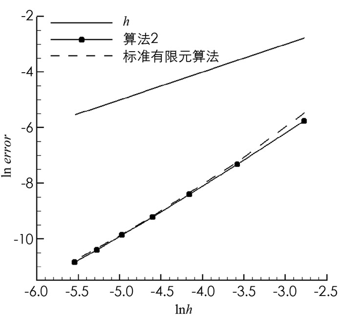
然后将每个子区域D_j向外扩展尺寸h得到Ω_j(j=1，2，3，4).计算时，取υ=0.01，迭代初值λ⁰=1，参数ρ=υ，使用P₁b-P₁元.算法2中细网格尺寸为$h=\frac{1}{n^{2}}(n=4, 6, \cdots, 16) $，粗网格与细网格尺寸关系满足$2 H=h^{\frac{1}{2}} $.表 1为标准有限元算法的数值结果，表 2为算法2的数值结果，其中，T为算法在4个子区域上计算时间的最大值，计算时间为网格生成时间、方程求解时间和误差计算时间之和. RuH¹和RpL²分别表示相对误差$\frac{\left\|\boldsymbol{u}-\boldsymbol{u}_{h}\right\|_{1, \mathit{\Omega}}}{\|\boldsymbol{u}\|_{1, \mathit{\Omega}}} $和$\frac{\left\|p-p_{h}\right\|_{0, \mathit{\Omega}}}{\|p\|_{0, \mathit{\Omega}}} $关于h的收敛率.对比表 1和表 2可知，算法2与标准有限元算法的收敛阶(如图 1，2)和近似解精度没有明显差别，但对比T可以看出算法2能节省大量的计算时间.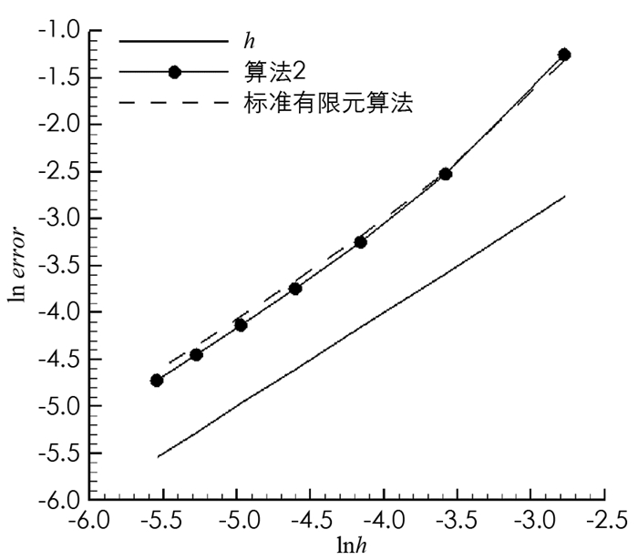

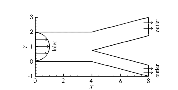
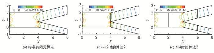
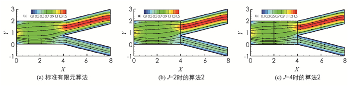
该算例研究了分叉动脉血管中血液流动的二维简化模型，假设血管为具有一定长度的“Y”字形管(图 3)，血液从左入口流入主血管再从两个分支血管流出，流入速度为u₁=1.2-1.2(y-1)²，u₂=0.设主血管的直径为2，主分支出口的宽度为1.25，另一个分支出口的宽度为0.75，在主血管的上、下边界取滑移边界，阈值函数g=|σ_τ|，其余的区域边界取Dirichlet边界.计算时使用P₂-P₁元，υ=1，应用Delaunay网格生成方法，细网格区域为每单位12个网格点，粗网格区域为每单位4个网格点.图 4-5分别为压力等值线、速度与流线的数值模拟图.图 4-5中，3组结果没有明显差别，压力在分叉连接处变化剧烈，速度在主分支血管内变化较大，并达到最大值.

基于完全区域分解法，本文设计并分析了一种求解带非线性滑移边界条件Stokes方程的并行有限元算法.通过数值算例，对比标准有限元算法，验证了并行有限元算法的有效性和高效性.